Cyclistic Bike Share Analysis

Overview

This project is my capstone case study for the Google Data Analytics Professional Certificate program. During it, I analyzed trip-level data from the Chicago based bike share service Divvy in the context of a fictional business called Cyclistic. Acting as a data analyst on a marketing team, I was tasked with answering the question: How do annual members and casual riders differ in their use of Cyclistic bikes?

Answering this question required me to engage in the entire data analytics process. The milestones of this project include:

1. Determining the business task and the set of deliverables which were expected of me as a data analyst.
2. Gathering the correct data sets which would be required to answer the core question.
3. Using the R programming language with R Studio to clean, process, analyze, and visualize my data.
4. Making sensible business recommendations based on the findings of my analysis.

To view the full source code of this project see the Kaggle Notebook.

The Scenario

You are a data analyst working for a Chicago based bike share company called Cyclistic. The company has a fleet of almost 6,000 bicycles that can be retrieved from and deposited at any of the approximately 700 stations spread throughout the city. Their pricing plan offers single-ride passes, full-day passes, and annual memberships. Customers who have annual memberships are referred to as “annual members”. All other customers are called “casual riders”.

The company’s financial analysts have determined that annual members are significantly more profitable than causal riders. Your manager, the director of marketing, believes that maximizing the number of annual members is the key to the company’s growth. Therefore, her goal is to design a marketing strategy which will convert casual riders into annual members.

To do this, the marketing team needs to answer three key questions:

• How do annual members and casual riders differ in their use of Cyclistic bikes?
• Why would a casual rider buy a Cyclistic annual memberships?
• How can Cyclistic use digital media to influence casual riders to become members?

Our manager has tasked us with answering the first of these three questions: How do annual members and casual riders differ in their use of Cyclistic bikes?

Findings

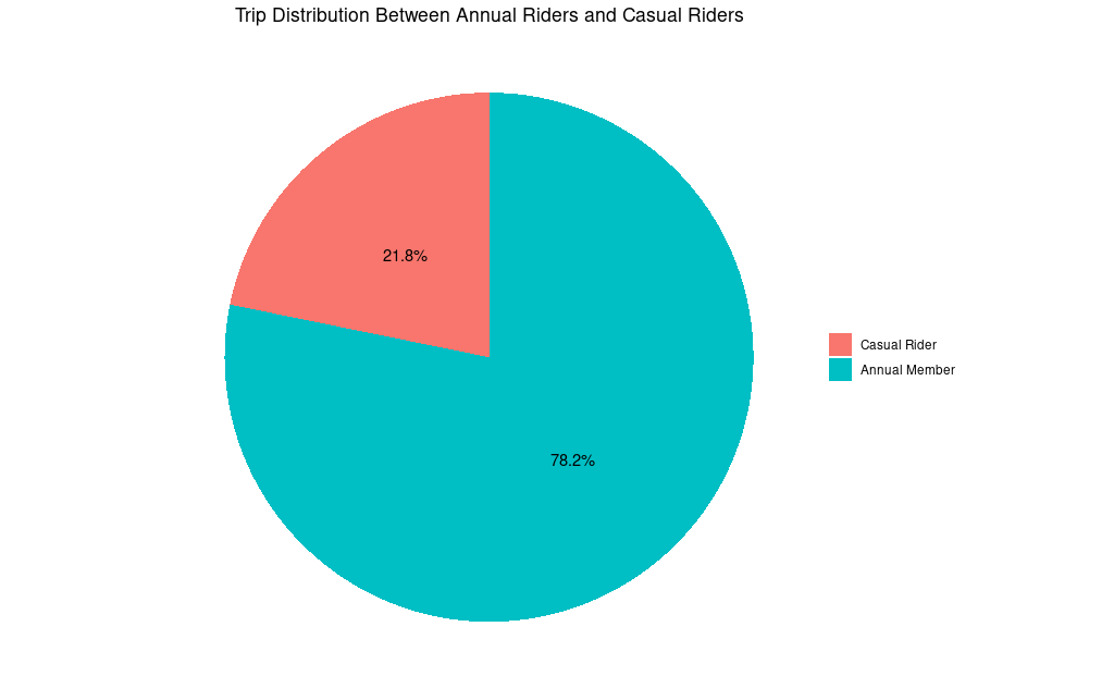
Through my analysis I was able to find several differences in the behavior of annual members and casual riders. Firstly, I found that casual riders are responsible for significantly less of the total number of bike share trips. In fact, casual riders accounted for only 21.8% of total bike trips. Meanwhile, usage by annual members was over three times higher and accounted for 78.2% of total bike trips.

There were also differences in when the two groups use the bike share service. Throughout the year, usage between the two groups was quite similar. Both groups go on less bike trips in the Winter and late Fall months. And, both groups go on more bike trips in the Spring and Summer months with peaks around August.

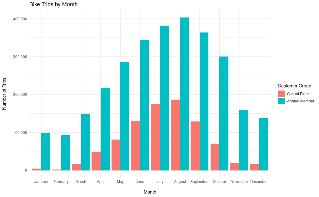
However, bike share usage by annual members is several times higher in Winter compared to casual riders. In November, December, January, and February, bike share trips by casual riders are almost non-existent. This indicates that there is some fundamental difference between the people composing the casual rider group compared to the annual member group.

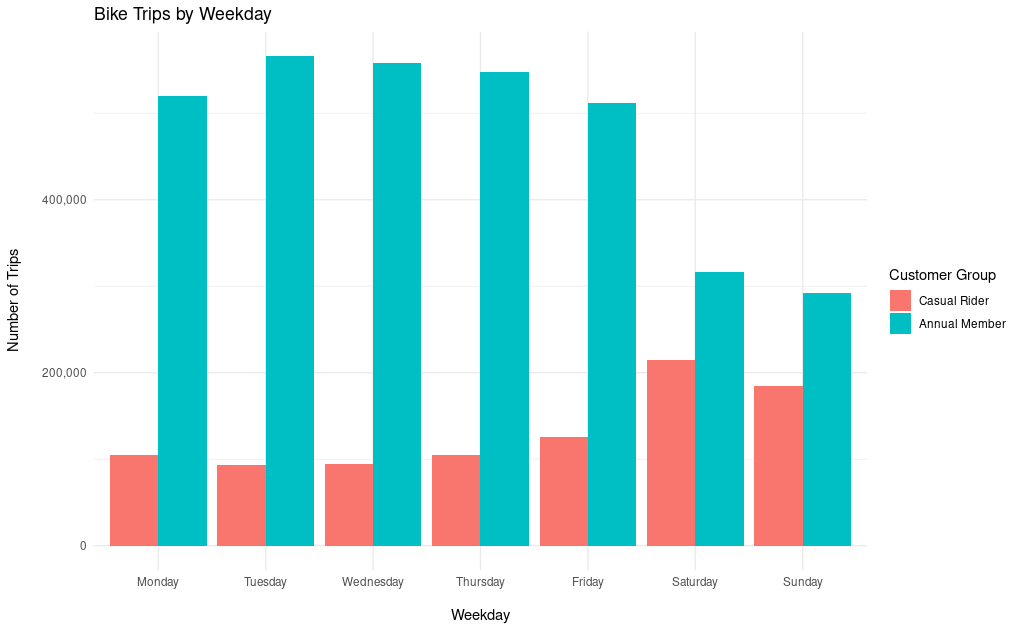
An analysis of which day of the week trips take place in each group gives us more insight. During the workweek, trips by casual riders are low. But, the number of trips they take rises on the weekend. The inverse is true for annual members. Annual members take many trips during the workweek. However, their usage drops during the weekend.

This could be explained in a number of ways. The most obvious is that the casual rider group is composed of more tourists than city residents. For example, the increase in trips by casual riders on the weekend could represent people coming into the city for weekend entertainment.

Additionally, the drastic fall in trips by casual riders during the Winter months could coincide with an overall decrease in tourism. The fact that trips by casual riders are extremely low in the Winter months, while trips by annual members remain relatively high, lends credence to the idea that the casual rider group contains less city residents.

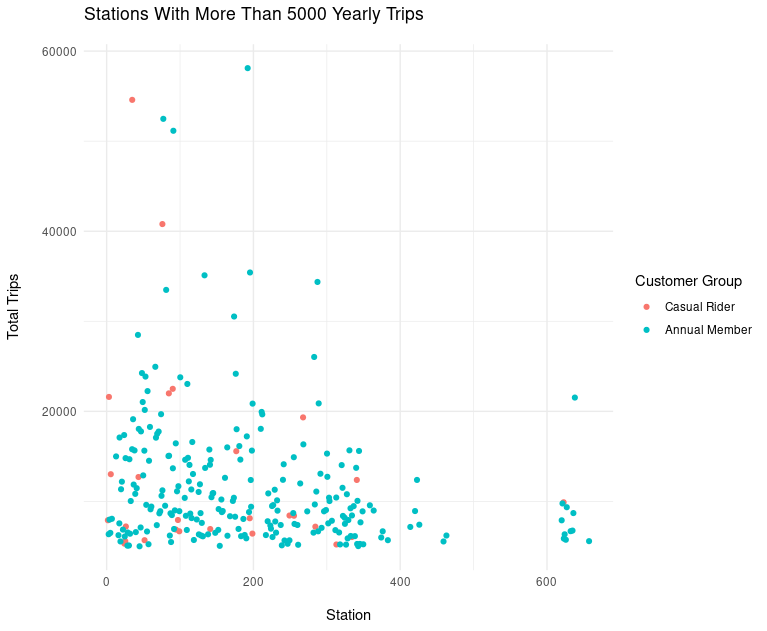
Investigating the overlap between which bike share stations each customer group uses also shows a fundamental behavioral difference.

In the above chart, we examine the trip totals by each customer group originating from stations with 5000 or more total trips. In other words, these are the most popular stations. As you can see, the most popular stations are not as popular with casual riders as they are with annual members.

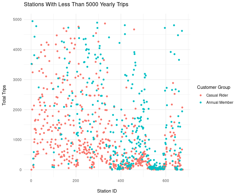
Likewise, if we examine stations with less than 5000 total trips, i.e. the unpopular stations, we find a greater degree of overlap. Additionally, there is a cluster of stations which are unpopular in both groups. This information might be help when deciding which stations to focus the marketing campaign upon.

Finally, there is one last descriptive element of our data worth noting. On average, annual members use their bike for just under 13 minutes, while casual riders use their for around 40 minutes.

Recommendations

Based on these findings, there are several recommendations to be made:

1. The marketing campaign should be limited to the Spring and Summer months. These are the months that recieve that greatest amount of activity from casual riders. The Fall months represent a sharp decline in bike share usage, and in the Winter months bike share usage is almost non-existent.

2. The marketing campaign should be intensified on the weekends. We know that casual riders tend to use the bike share more on the weekend than during the workweek. While usage during the workweek is fairly level in the casual rider group, it spikes on Saturday and Sunday, so it makes sense to spend more on marketing during this time period.

3. The marketing campaign should focus on stations popular with casual riders. We know from our analysis that the stations which casual riders use differ from annual riders. Targeting the top stations would result in targeting predominately existing annual riders. Instead, focusing on stations popular with casual riders is likely to be more effective.

4. Perform further information gathering on the casual rider customer group. Given the behavioral differences between casual riders and annual members, it seems likely that casual riders are fundamentally different in some way. The casual riders most likely to be converted to annual members are either frequents tourists or city residents who have not yet purchased an annual subscription. By finding out more about who the casual riders are as people, perhaps through a survey, we can better market the service to them.

Methods

This section contains the data analytics notebook which was a required deliverable for the capstone project. This section is more technical than the proceeding section, and serves as a record of the cleaning, processing, and analytic methods I used to arrive at the findings and recommendations shared above. Below you will find a more detailed explanation of the data used in this project, the challenges faced when cleaning and processing it, and the analytical methods used to arrive at my conclusions.

Gathering Our Data

The company’s internal data is broken down into quarterly chunks. We have access to CSV data from the first quarter of 2015 to the first quarter of 2020. Our task is to analyze how bike use differs between annual members and casual riders, so we are only interested in data that informs us about recent usage trends. Therefore, we will focus our analysis on the data from 2019 and 2020.

For this project I used the four quarters from 2019 and the first quarter from 2020 which can be downloaded here. Download the following zip files:

• Divvy_Trips_2019_Q1.zip
• Divvy_Trips_2019_Q2.zip
• Divvy_Trips_2019_Q3.zip
• Divvy_Trips_2019_Q4.zip
• Divvy_Trips_2020_Q1.zip

Each of these zip files contains a corresponding CSV file which contains the data needed for our analysis.

Note: The data we are using is provided by Divvy for public use.

Data Cleaning

Now that we know our business task and have the data, our next step is to clean and process the data so that it can be used for analysis. We will start by loading our data files into memory. In the code below, we load every CSV files in the file_paths list into a list of five data frames called data_files.

 1
 2
 3
 4
 5
 6
 7
 8
 9
10

# A list of file paths to our data files.
file_paths <- list(
  "data/2019_Q1.csv",
  "data/2019_Q2.csv",
  "data/2019_Q3.csv",
  "data/2019_Q4.csv",
  "data/2020_Q1.csv")

# Load all data files in the file_paths list into a list of data frames
data_files <- lapply(file_paths, read.csv, stringsAsFactors = FALSE)

Our first goal in the cleaning process is to integrate the data for our five data frames into a single data frame. Before we can do this we must first review and verify the integrity of our data.

Upon first inspection of the loaded data it is clear that there are some inconsistencies that must be fixed. The Q1, Q3, and Q4 data sets for 2019 seem to be fairly consistent. Each data frame contains the following columns:

The second quarter of 2019 has all the same types of data, but uses different column names. We will apply the column names from the first quarter of 2019 to all other quarters in 2019 to ensure consistent naming across the entire 2019 data set.

1
2
3
4

# Applies the columns from the first quarter of 2019 to the second, third, and fourth quarters of 2019.
colnames(data_files[[2]]) <- colnames(data_files[[1]])
colnames(data_files[[3]]) <- colnames(data_files[[1]])
colnames(data_files[[4]]) <- colnames(data_files[[1]])

The first quarter of 2020 is a far more complicated case. Here is its structure:

Not only does it use different column names, but it also missing certain columns such as gender, birthyear, and tripduration. Additionally, it contains data that other data set don’t have such as the starting and ending longitude and latitude, and bike type. Finally, there are some data type inconsistencies.

If our current goal is to map the five data frames into one unified data frame for further analysis we will have to:

• Rename the columns we are keeping to the standard column names.
• Remove the unwanted columns.
• Add in missing columns filled will NA data.
• Calculate a tripduration column.
• Fix any data type inconsistencies.

The following will do just that.

 1
 2
 3
 4
 5
 6
 7
 8
 9
10
11
12
13
14
15
16
17
18
19
20
21
22
23
24
25
26
27
28
29
30
31
32
33
34

# Rename the columns we are keeping
names(data_files[[5]])[1] <- 'trip_id'             # Rename ride_id to trip_id
names(data_files[[5]])[3] <- 'start_time'          # Rename started_at to start_time
names(data_files[[5]])[4] <- 'end_time'            # Rename ended_at to end_time
names(data_files[[5]])[5] <- 'from_station_name'   # Rename start_station_name to from_station_name
names(data_files[[5]])[6] <- 'from_station_id'     # Rename start_station_id to from_station_id
names(data_files[[5]])[7] <- 'to_station_name'     # Rename end_station_name to to_station_name
names(data_files[[5]])[8] <- 'to_station_id'       # Rename end_station_id to to_station_id
names(data_files[[5]])[13] <- 'usertype'           # Rename member_casual to usertype

# Remove the columns we don't want
data_files[[5]]$rideable_type <- NULL
data_files[[5]]$start_lat <- NULL
data_files[[5]]$start_lng <- NULL
data_files[[5]]$end_lat <- NULL
data_files[[5]]$end_lng <- NULL

# Add the missing columns filled with NA data (bind_rows from dply might do this
# automatically, but I included it to be more explicit).
data_files[[5]]$gender <- as.character(NA)
data_files[[5]]$birthyear <- as.integer(NA)
data_files[[5]]$bikeid <- as.integer(NA)

# Rename usertype values (member -> Subscriber AND causal -> Customer)
data_files[[5]] <- data_files[[5]] %>%
  mutate(usertype = recode(usertype, "member" = "Subscriber", "casual" = "Customer"))

# Calculate the tripduration. We store it as a character type because that is how 
# it is in the 2019 data frames and this can be easily converted to integer or numeric
# types if/when we need to.
data_files[[5]]$tripduration <- as.character(
  as.POSIXct(data_files[[5]]$end_time, format="%Y-%m-%d %H:%M:%S") - 
  as.POSIXct(data_files[[5]]$start_time, format="%Y-%m-%d %H:%M:%S")
)

Our 2020 Q1 data is now ready. The last step before mapping our data into a single data frame is to fix any inconsistencies between data types. The only column of concern is trip_id which is stored as integers in the 2019 data, but as characters in the 2020 data. We will convert all trip_ids from 2019 into characters.

1
2
3
4

data_files[[1]] <- data_files[[1]] %>% mutate(trip_id = as.character(trip_id))
data_files[[2]] <- data_files[[2]] %>% mutate(trip_id = as.character(trip_id))
data_files[[3]] <- data_files[[3]] %>% mutate(trip_id = as.character(trip_id))
data_files[[4]] <- data_files[[4]] %>% mutate(trip_id = as.character(trip_id))

Finally, we can combine the five data frames together using bind_rows() from the dplyr library.

1

bike_trip_data <- bind_rows(data_files[[1]], data_files[[2]], data_files[[3]], data_files[[4]], data_files[[5]])

Now that we have a single data frame containing the fully integrated bike trip data, we want to continue the process of cleaning our data by performing a descriptive analysis. This will help us get a better picture of our overall data set. It will also assist in the cleaning process by finding potential errors in our data. To perform our descriptive analysis we will systematically go through each column and investigate it for issues.

To begin, we will transform any empty strings in our data frame into NA types:

1

bike_trip_data[bike_trip_data == ""] <- NA

This will help make our data set more consistent overall. Next, we will make sure that trip_id only contains unique values:

1

anyDuplicated(bike_trip_data$trip_id)

There are no duplicates, and we wouldn’t be able to rectify any missing trip ids, so we can move on to the start_time and end_time columns.

First, we should convert start_time and end_time data into POSIXct data types instead of characters so that they are easier to work with.

1
2

bike_trip_data$start_time <- as.POSIXct(bike_trip_data$start_time, format = "%Y-%m-%d %H:%M:%S")
bike_trip_data$end_time <- as.POSIXct(bike_trip_data$end_time, format = "%Y-%m-%d %H:%M:%S")

Next, let’s look for any NA or NULL rows in the start_time and end_timecolumns.

1
2
3
4

bike_trip_data[is.na(bike_trip_data$start_time), ]
bike_trip_data[is.na(bike_trip_data$end_time), ]
bike_trip_data[sapply(bike_trip_data$start_time, is.null), ]
bike_trip_data[sapply(bike_trip_data$end_time, is.null), ]

No rows are found to contain NA or NULL values. Now, we can make sure that there are no end times that are earlier than start times.

1
2

# Get the indices for any row in which the end_time is earlier than the start_time
idx <- which(bike_trip_data$end_time < bike_trip_data$start_time) 

Unfortunately, there are 130 rows in which end_time is earlier than start_time. We have to make a choice about how to handle this problem. We could swap the end_time and start_time in the rows, but we would first have to make sure that the rest of the data they contain is valid. Given the size of our dataset, I think it is safe simply to exclude these rows.

1
2

# Drop the rows in which end_time is earlier than start_time
bike_trip_data = bike_trip_data[-c(idx), ]

Now we can move onto tripduration. This column might be very important to answering our question, so its important that is it properly formatted. Let’s recalculate tripduration using start_time and end_time, but store it in a new column called new_trip_duration:

1

bike_trip_data$new_trip_duration <- bike_trip_data$end_time - bike_trip_data$start_time;

Now, let’s investigate the qualities of this new_trip_duration to see if there are any problems.

1
2
3

max(bike_trip_data$new_trip_duration) # 10628422 seconds, or 123 days
mean(bike_trip_data$new_trip_duration) # 1438 seconds which seems fairly accurate
min(bike_trip_data$new_trip_duration) # 0 seconds which might be normal

The max, mean, and min values all return reasonable results. There are some outliers. For example, the longest trip is over three months long, which could be an error or indicate a missing or stolen bike. Additionally, some trips are only a few seconds long. This data isn’t inherently problematic, but we might consider removing it before we begin our analysis.

Next, we will take a look at the from_station_id and to_station_id columns. We start by checking it for NA or NULL values, and checking the max and min values:

 1
 2
 3
 4
 5
 6
 7
 8
 9
10

# Checks for NA or NULL values
bike_trip_data[is.na(bike_trip_data$from_station_id), ]
bike_trip_data[is.na(bike_trip_data$to_station_id), ]
bike_trip_data[sapply(bike_trip_data$from_station_id, is.null), ]
bike_trip_data[sapply(bike_trip_data$to_station_id, is.null), ]

max(bike_trip_data$from_station_id)
max(bike_trip_data$to_station_id)
min(bike_trip_data$from_station_id)
min(bike_trip_data$to_station_id)

Everything checks out. There are no NA or NULL values, and the min and max are identical for each (1 and 675).

Processing the Data

At this point, the original data sets we received have been integrated into a single data frame, and the original data has been cleaned. This is a good point to return to our business question, and consider what types of data we might be able to derive from our existing data to better complete our business task.

The question we are trying to answer is: How do annual members and casual riders differ in their use of Cyclistic bikes?

In our existing data, the usertype and tripduration fields are likely to provide some insight into the differences between annual members and casual riders. However, we can extract even more useful information from fields such as start_time and end_time. For example, we can determine which day of the week a trip starts and ends on to see if causal riders and annual members use their bikes during different times.

We will do this by storing each trip’s starting and ending weekday in the start_weekday and end_weekday columns:

1
2

bike_trip_data$start_weekday <- weekdays(bike_trip_data$start_time)
bike_trip_data$end_weekday <- weekdays(bike_trip_data$end_time)

We might also benefit from extracting the month, year, and quarter from the start_time and end_time fields and storing them as dedicated attributes.

 1
 2
 3
 4
 5
 6
 7
 8
 9
10
11

# Extract the month from the start and end times
bike_trip_data$start_month <- format(bike_trip_data$start_time, "%B")
bike_trip_data$end_month <- format(bike_trip_data$end_time, "%B")

# Extract the year from the start and end times
bike_trip_data$start_year <- format(bike_trip_data$start_time, "%Y")
bike_trip_data$end_year <- format(bike_trip_data$end_time, "%Y")

# Extract the quarter
library(lubridate)
bike_trip_data$quarter <- quarter(bike_trip_data$start_time)

If we want to be extra verbose, we could also convert the new_trip_duration field into different time scales. For example, instead of only having trip duration in seconds, we could calculate it in minutes, hours, and days:

1
2
3
4
5

library(lubridate)

bike_trip_data$duration_in_minutes <- as.duration(bike_trip_data$new_trip_duration) / dminutes(1)
bike_trip_data$duration_in_hours <- as.duration(bike_trip_data$new_trip_duration) / dhours(1)
bike_trip_data$duration_in_days <- as.duration(bike_trip_data$new_trip_duration) / ddays(1)

With that complete, we are finished cleaning and processing our dataset. Our data should be of a reasonable enough quality to perform the analysis required of us.

We will save our cleaned dataset as an .RData file.

1
2
3
4
5
6
7
8

# Save as an RData file to retain type information
save(bike_trip_data, file = "data/bike_trip_data_2019_Q1_through_2020_Q1_CLEANED.RData")

# Optionally save it as a CSV, but you will lose type information
write.csv(bike_trip_data, "data/bike_trip_data_2019_Q1_through_2020_Q1_CLEANED.csv")

# You can load the RData file with
load("data/bike_trip_data_2019_Q1_through_2020_Q1_CLEANED.RData")

Performing the Analysis

Now that we have a workable data set we can begin the process of analysis. The question we are tasked with answering is: How do annual members and casual riders differ in their use of Cyclistic bikes? In other words, using the data we have we want to determine how the usage of the Cyclistic bike share service differs between annual members and casual riders. And, we want to use that analysis to provide insight to are stakeholders, in this case the marketing director and team, which will inform their marketing campaign.

Immediately, a few angles of analysis come to mind:

• How do the number of annual members compare to casual riders?
• Do different user types ride more on different days of the week?
• Does the average trip duration differ between annual members and casual riders?
• Do certain stations have a higher concentration of annual members or casual riders?
• Is there a difference between the time of day, or year, when annual members or casual riders use the service?

Before we attempt to gain insight into some of these questions, it is important to determine which subset of our data we will be using. A basic analysis of our user’s trip duration tells us a few things:

1
2
3

max_duration_in_days <- as.numeric(max(bike_trip_data$duration_in_days))
min_duration_in_days <- as.numeric(min(bike_trip_data$duration_in_days))
mean_duration_in_days <- as.numeric(mean(bike_trip_data$duration_in_days))

Firstly, we know that our data set contains some odd trip durations. There are trip durations which last many months, which may indicate either an error in the system or a bike which was missing or stolen, and there are trip durations which last no time at all (zero seconds, or are otherwise very short). Because we are examining the differences in behavior between customers groups who use the bike service, it is reasonable to exclude anomalous trip data (such as those that are very long and those that are very short).

Therefore, it is reasonable to limit our data set to trips that are at least one minute and at most forty-eight hours. We will store this data set in filtered_bike_data:

filtered_bike_data <- subset(bike_trip_data, duration_in_minutes > 1 & duration_in_minutes < 2880)

With our filtered data set, we can being our analysis in earnest. The first question to investigate is the ratio of annual member trips to casual riders. A good chart type to give an intuitive understanding of that ratio is a pie chart:

 1
 2
 3
 4
 5
 6
 7
 8
 9
10
11
12
13
14
15
16
17
18
19
20
21
22

library(tidyverse)
library(ggplot2)
library(dplyr)

# Create a summary of the counts per usertype
user_counts <- as.data.frame(table(filtered_bike_data$usertype))
colnames(user_counts) <- c("usertype", "count")

# Calculate count percentages
user_counts$percent <- round(100 * user_counts$count / sum(user_counts$count), 1)

# Create a pie chart
ggplot(user_counts, aes(x= "", y = count, fill = usertype)) +
  geom_bar(width = 1, stat = "identity") +
  coord_polar(theta = "y") +
  geom_text(aes(label = paste0(percent, "%")),
            position = position_stack(vjust = 0.5)) +
  theme_void() +  # Removes axes and gridlines
  theme(legend.title = element_blank()) +
  theme(plot.title = element_text(hjust = 0.5)) +
  labs(title = "Trip Distribution Between Annual Riders and Casual Riders") + 
  scale_fill_discrete(labels = c("Casual Rider", "Annual Member"))

The result of our pie chart tells us that about 78% of all trips are taken by annual members. Meanwhile, casual riders, the group we are trying to convert into subscribers, make up only 22% of our group. Next, we should investigate, the days of the week annual members use the bike share service compared to casual riders.

 1
 2
 3
 4
 5
 6
 7
 8
 9
10
11
12
13
14
15

library(scales)
library(ggplot2)

ggplot(filtered_bike_data, aes(x = start_weekday, fill = usertype)) +
  geom_bar(position = "dodge") +  # dodge places bars side by side
  labs(title = "Bike Trips by Weekday",
       x = "Weekday",
       y = "Number of Trips",
       fill = "Customer Group") +
  theme_minimal() +
  theme(axis.title.x = element_text(margin = margin(t = 15))) +
  theme(axis.title.y = element_text(margin = margin(r = 15))) +
  scale_x_discrete(limits = c("Monday","Tuesday","Wednesday","Thursday","Friday","Saturday","Sunday")) +
  scale_fill_discrete(labels = c("Casual Rider", "Annual Member")) +
  scale_y_continuous(labels = comma)

From this bar chart we can compare the trends in each customer group by the weekday. We see that the number of casual riders increases on Friday, peaks on Saturday and Sunday, and then hits a low during the middle of the workweek. The annual rider usage is the inverse. Usage peaks during the middle of the workweek, and it sharply falls to a low on the weekends.

This indicates that some portion of the annual customers are likely using the bike share service as a a way to commute. While casual riders tend to use the bike share on the weekends. This might mean that casual riders have a higher number of tourists in the group, or that residents who are not subscribed only use the bikes when not working.

A recommendation is beginning to form. We know that just under a quarter of the total bike share customers are casual riders. And, we know that bike share usage by casual riders is lowest during the workweek and highest during the weekend. We should investigate further by checking how bike share usage differ on a month-to-month basis. After that, we might want to check how the duration of bike share usage differs between casual and annual riders. And then analyze stations to see if certain stations are more popular among casual riders.

First, let’s see how bike share usage differs in each group on a month-to-month basis:

 1
 2
 3
 4
 5
 6
 7
 8
 9
10
11
12
13
14
15
16
17
18

library(ggplot2)
library(scales)

filtered_bike_data_2019 <- subset(filtered_bike_data, start_year == 2019)

ggplot(filtered_bike_data_2019, aes(x = start_month, fill = usertype)) +
  geom_bar(position = "dodge") + 
  labs(title = "Bike Trips by Month",
       x = "Month",
       y = "Number of Trips",
       fill = "Customer Group") +
  theme_minimal() +
  theme(axis.title.x = element_text(margin = margin(t = 15))) +
  theme(axis.title.y = element_text(margin = margin(r = 15))) +
  scale_x_discrete(limits = c("January","February","March","April","May","June",
                              "July","August","September","October","November","December")) +
  scale_fill_discrete(labels = c("Casual Rider", "Annual Member")) +
  scale_y_continuous(labels = comma)

This bar chart is quite revealing about the behavior of casual riders. Annual riders tend to use the bike share service consistently across the entire year. There is an obvious rise through Spring and peak in late Summer. However, casual riders use the service significantly less in the Winter months compared to annual riders. Like the annual riders their usage rises through Spring, peaks in Summer, and drops in Fall.

This indicates that if we were going to be advertising to them we would want to target these advertisements during the Spring and Summer months.

We are starting to get a good idea about the differences between annual members and casual riders. We know that both groups’ usage declines in the Fall and Winter, rises in the Spring, and peaks towards the end of the Summer. Furthermore, we know that casual riders tend to use the bikes less during the workweek and more on the weekend.

Next, we should do some basic investigation of the two groups’ trip durations and top starting and ending bike stations. To do this, we will create two new data frames, each containing only annual riders or casual riders:.

1
2

annual_riders <- filtered_bike_data[filtered_bike_data$usertype == "Subscriber", ]
casual_riders <- filtered_bike_data[filtered_bike_data$usertype == "Customer", ]

Next, we will compare the mean duration_in_minutes of each groups:

1
2

annual_rider_mean_trip_duration <- mean(annual_riders$duration_in_minutes)
casual_rider_mean_trip_duration <- mean(casual_riders$duration_in_minutes)

This gives us an interesting result. Despite both data sets being limited to trips with a minimum time of one minute, and a maximum time of two days, casual riders use their bikes for three times as long as annual members. Specifically, casual riders use bikes on average for around 40 minutes. Annual riders use their bikes for only 13 minutes on average.

Let’s check the two data sets to see if trips over one day in length is more common than in the other.

1
2

sum(annual_riders$duration_in_days >= 1)
sum(casual_riders$duration_in_days >= 1)

In our data, casual riders had 696 trips over a day in length while annual riders had only 315 trips lasting over a day. Let’s filter out all trips longer than a day from our data set, and reassess the mean duration_in_minutes

 1
 2
 3
 4
 5
 6
 7
 8
 9
10
11
12
13
14
15

filtered_bike_data <- subset(filtered_bike_data, filtered_bike_data$duration_in_days <= 1)
annual_riders <- filtered_bike_data[filtered_bike_data$usertype == "Subscriber", ]
casual_riders <- filtered_bike_data[filtered_bike_data$usertype == "Customer", ]

annual_rider_mean_trip_duration <- mean(annual_riders$duration_in_minutes)
casual_rider_mean_trip_duration <- mean(casual_riders$duration_in_minutes)

# You can save the annual and casual riders data frames for later use.
# REMEMBER: This data set as been filtered to include only trips greater than a minute
# in duration and less than or equal to a day. 
save(annual_riders, file = "data/annual_rider_bike_data_2019_Q1_through_2020_Q1_CLEANED.RData")
save(casual_riders, file = "data/casual_rider_bike_data_2019_Q1_through_2020_Q1_CLEANED.RData")

load("data/annual_rider_bike_data_2019_Q1_through_2020_Q1_CLEANED.RData")
load("data/casual_rider_bike_data_2019_Q1_through_2020_Q1_CLEANED.RData")

The values are basically the same: 12.7 minutes for annual riders and 39.4 minutes for casual riders. This tells us important information about how the two customer groups use the bike share. Annual riders use their bikes for less time, but perhaps more frequently, while casual riders use their bikes for longer, but make up a smaller quantity of the total trips taken.

Our last angle of analysis will be around bike stations. We will look at our two groups and compare their top stations for both starting and ending trips.

 1
 2
 3
 4
 5
 6
 7
 8
 9
10
11
12

library(dplyr)
top_from_stations_casual <- casual_riders %>% 
  count(from_station_name, sort = TRUE)
  
top_to_stations_casual <- casual_riders %>% 
  count(to_station_name, sort = TRUE)
  
top_from_stations_annual <- annual_riders %>% 
  count(from_station_name, sort = TRUE)
  
top_to_stations_annual <- annual_riders %>% 
  count(to_station_name, sort = TRUE)

An analysis of the top ten stations for each customer group is quite revealing. The stations that casual customers use are all located in tourist heavy areas such as the South Loop, while annual rider’s top stations tend to be in the West loop which is a business district.

 1
 2
 3
 4
 5
 6
 7
 8
 9
10
11
12
13
14
15
16
17
18
19
20
21
22
23
24
25
26
27
28
29
30
31
32
33
34
35
36

library(ggplot2)
library(dplyr)
library(tidyr)

top_from_stations_casual$usertype <- "Customer"
top_from_stations_annual$usertype <- "Subscriber"

combined <- bind_rows(top_from_stations_casual, top_from_stations_annual )

sorted_combined <- combined %>% 
  arrange(desc(n)) %>% 
  slice_head(n = 100)

total_combined <- sorted_combined %>%
  group_by(from_station_name) %>%
  mutate(total = sum(n)) %>%
  ungroup()

ggplot(total_combined, aes(x = reorder(from_station_name, -total), y = n, fill = usertype)) +
  geom_bar(stat = "identity") +
  labs(
    title = "Station Usage by Customer Type",
    x = "Station",
    y = "Number of Customers",
    fill = "Customer Type"
  ) +
  theme_minimal() +
  theme(
    axis.ticks.x = element_blank(),
    axis.text.x = element_blank(),
    panel.grid.major = element_blank(),
    panel.grid.minor = element_blank(),
  ) +
  theme(axis.title.x = element_text(margin = margin(t = 15))) +
  theme(axis.title.y = element_text(margin = margin(r = 15))) +
  scale_fill_discrete(labels = c("Casual Rider", "Annual Member"))

The geographic seperation Finally, let’s make some scatterplots to show the distribution of starting station trip totals between each customer group.

 1
 2
 3
 4
 5
 6
 7
 8
 9
10
11
12
13
14
15
16
17
18
19
20
21
22
23
24
25
26
27
28
29
30
31
32
33
34
35
36
37
38
39
40
41
42
43
44
45
46
47
48
49
50
51
52
53
54
55
56
57
58
59

library(dplyr)
library(ggplot2)
library(patchwork)

# Find the total number of trips for each station used by casual riders
casual_stations <- casual_riders %>% 
  group_by(from_station_id) %>% 
  summarise(count = n()) %>% 
  mutate(usertype = "Customer")
  
# Find the total number of trips for each station used by annual members
annual_stations <- annual_riders %>% 
  group_by(from_station_id) %>% 
  summarise(count = n()) %>%
  mutate(usertype = "Subscriber")

# Combine stations and filter based on trip count
combined_stations <- bind_rows(casual_stations, annual_stations)
popular_stations <- combined_stations %>% 
  filter(count >= 5000)

unpopular_stations <- combined_stations %>% 
  filter(count <= 5000)
  
# Create a scatterplot of stations with more than 5000 year trips
ggplot(popular_stations, aes(
    x=from_station_id, 
    y=count,
    color=usertype
  )) +
  geom_jitter() +
  labs(
    title = "Stations With More Than 5000 Yearly Trips",
    x = "Station",
    y = "Total Trips",
    color = "Customer Group"
  ) +
  theme_minimal() +
  theme(axis.title.x = element_text(margin = margin(t = 15))) +
  theme(axis.title.y = element_text(margin = margin(r = 15))) +
  theme(plot.title = element_text(margin = margin(b = 15)))

# Create a scatterplot of stations with less than 5000 year trips
ggplot(unpopular_stations, aes(
    x=from_station_id, 
    y=count,
    color=usertype
  )) +
  geom_jitter() +
  labs(
    title = "Stations With Less Than 5000 Yearly Trips",
    x = "Station ID",
    y = "Total Trips",
    color = "Customer Group"
  ) +
  theme_minimal() +
  theme(axis.title.x = element_text(margin = margin(t = 15))) +
  theme(axis.title.y = element_text(margin = margin(r = 15))) +
  theme(plot.title = element_text(margin = margin(b = 15)))